
In a previous post, I wrote about how we use Multi-Armed Bandits to run adaptive A/B tests in our CRM platform. That post ended with a promise about smarter rewards and contextual bandits. What actually came next was something different - and, I think, more interesting: we stopped treating an email as a single thing to test.
An email is not an atom. It's a molecule: a subject line, a sender name, a title, a call-to-action, a body text. When you A/B test whole emails, you're testing combinations of those parts - and combinations multiply fast. This series is the story of Dynamic Templates: emails assembled at send time from per-slot variant pools, each slot optimized by its own bandit. Part 1 covers the core idea and the architecture that makes it safe.
This is a three-part series:
- Part 1 (this one): the concept, the combinatorial wall, and the architecture - where weights live, how sends read them, and the shape of the feedback loop.
- Part 2: the allocation strategies - probability matching vs proportional rules, the math and failure modes of each, how to choose a reward per slot, and the conditions that make Thompson Sampling safe to run in production.
- Part 3: the lifecycle - how to know when a test is done, statistical verdicts, promoting winners, and retiring a finished experiment into a plain template.
From A/B Variants to Templates with Slots
Classic A/B testing in a CRM tool looks like this: you write two (or five) complete emails, split the traffic, and wait. It works, but it has an awkward property - every variant is a full email. If you want to test three subject lines and two CTA buttons, you either write six full emails (every combination, by hand) or you test them sequentially and hope the learnings compose.
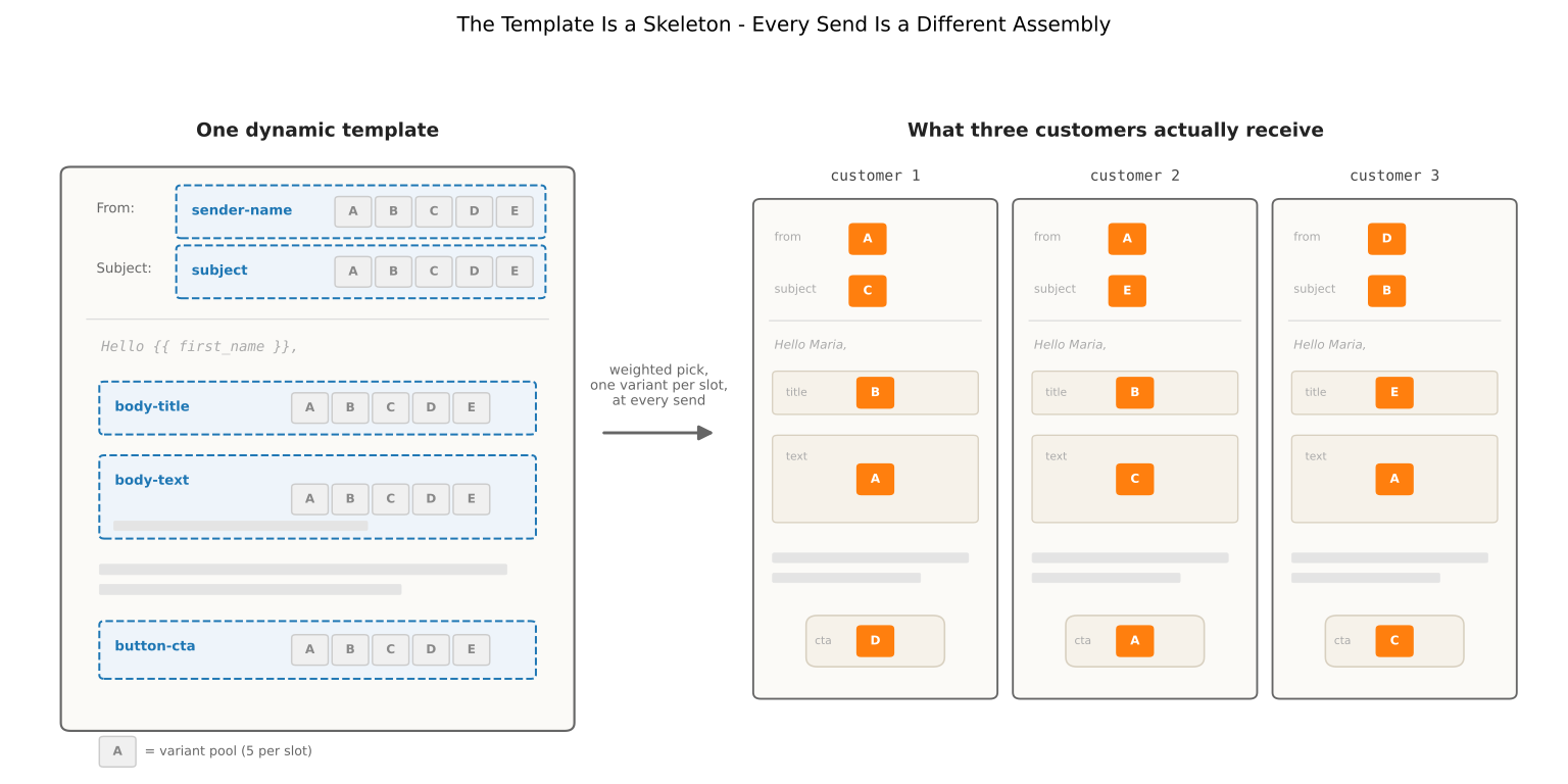
A dynamic template flips this around. The template itself has slots - placeholders for the parts we want to test: the subject line, the sender name, the body title, the body text, the CTA button. Each slot has a pool of variants - say, five subject lines, five titles, five CTAs. At send time, the system picks one variant per slot and assembles the final email. Every customer potentially receives a different combination, and every send is tagged with exactly which variant filled each slot, so the performance data flows back at the component level, not the email level.
The Combinatorial Wall
Here's the problem that makes per-slot testing genuinely different from whole-email testing, and not just cosmetically nicer.
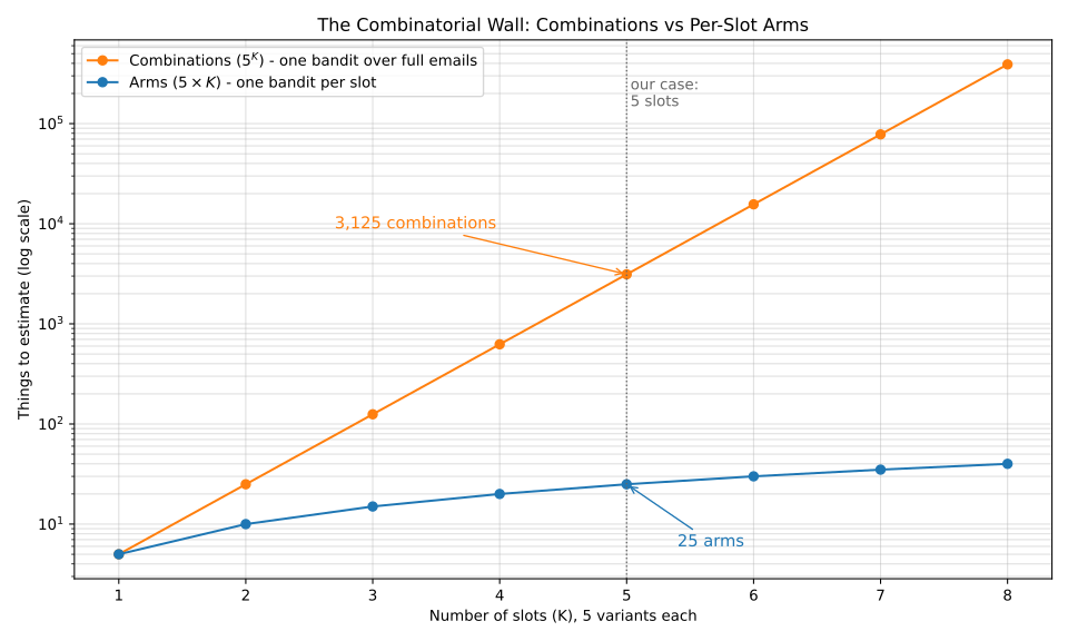
Say a template has $K = 5$ slots with $V = 5$ variants each. The number of distinct emails the system can assemble is:
$$V^K = 5^5 = 3{,}125$$
If you treat each combination as an arm of one big bandit - the "correct" formulation, in some sense - you need enough data per combination to rank them. Our optimizer keeps a component in uniform exploration until every arm has at least 500 sends (more on cold-start gates in Part 2). For 3,125 arms, that's over 1.5 million sends before the system is even allowed to start concluding anything. For a typical campaign audience, that's not slow learning - that's never learning. And it gets exponentially worse with every slot you add.
So we don't do that. Instead, we assume slots are independent and decompose the problem: five separate bandits, each with five arms.
$$V \times K = 5 \times 5 = 25 \text{ arms instead of } 3{,}125$$
That's a ~125× reduction in the number of things to estimate. But the decomposition is even better than that ratio suggests, because of sample reuse: every email sent is simultaneously a trial in all five bandits at once. One send gives the subject bandit one observation, the title bandit one observation, the CTA bandit one observation, and so on. In the combination formulation, that same send fed exactly one arm out of 3,125.
Of course, independence is an assumption. Since the system mixes the slots freely at send time, a variant that only works in one pairing - a "50% off!" subject on a body that never mentions the discount - is exactly the kind of interaction the decomposition can't see: each slot is judged on its marginal performance, averaged over whatever the other slots happened to serve alongside it.
In practice this stays cheap for two reasons:
- An authoring contract. Because any combination can ship, whoever builds the pools keeps every variant coherent with every variant of the other slots - so the self-contradicting pairings mostly never enter the pool to begin with.
- Interactions are second-order. Where they do slip through, they're small next to the main effects of a good subject or a good CTA - and modeling them explicitly would cost exactly the combinatorial wall we're trying to escape.
In Part 2, we'll see how the reward design makes this assumption tighter than it first appears.
Measure, Reward, Reallocate
With the slots decomposed into independent bandits, the whole feature runs one simple loop. We measure how each variant performs; a reward turns those measurements into an allocation - a set of percentages, one per variant; and at send time those percentages decide how much volume each variant gets. Better variants earn more volume, and because the loop recomputes every few hours as fresh opens and clicks arrive, the allocation keeps chasing the evidence.
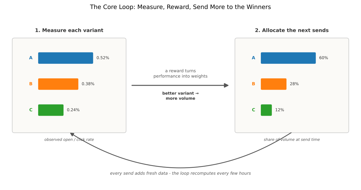
That's the entire idea. Everything else in this post is about running that loop safely - where the numbers live, how a send behaves when they're missing, and how the measurement actually reaches the optimizer. (How the reward itself turns counts into an allocation - the statistically interesting part - is all of Part 2.)
The Feedback Loop
The last piece is the loop that retunes the weights - and the measurement pipeline that feeds it. Every tracking event of every email (send, delivery, open, click) is tagged with the variant IDs that filled each slot and flows through the same real-time pipeline from the Multi-Armed Bandits post: Amazon SES emits the events through SNS into a Kinesis stream, a Databricks streaming job lands them in Delta within about a minute, and the medallion layers aggregate everything into a gold table of 30-day counts at the (action, slot, variant) grain - sent, opened, clicked, per variant, per slot. That table is the optimizer's entire view of the world.
The loop itself is a scheduled job that runs every 3 hours - the reward is delayed anyway (clicks trickle in for hours after a send), so recomputing faster would buy little, and bandit allocation is robust to slightly stale weights. Each run reads the gold, recomputes every action's distribution, and appends a new version to the weights table - of which it is the sole writer. After the initial uniform seed there is no hand-tuning; to intervene, you remove a variant or declare a winner (both in Part 3). The algorithm inside the loop is Part 2's whole subject; what matters here is the shape:
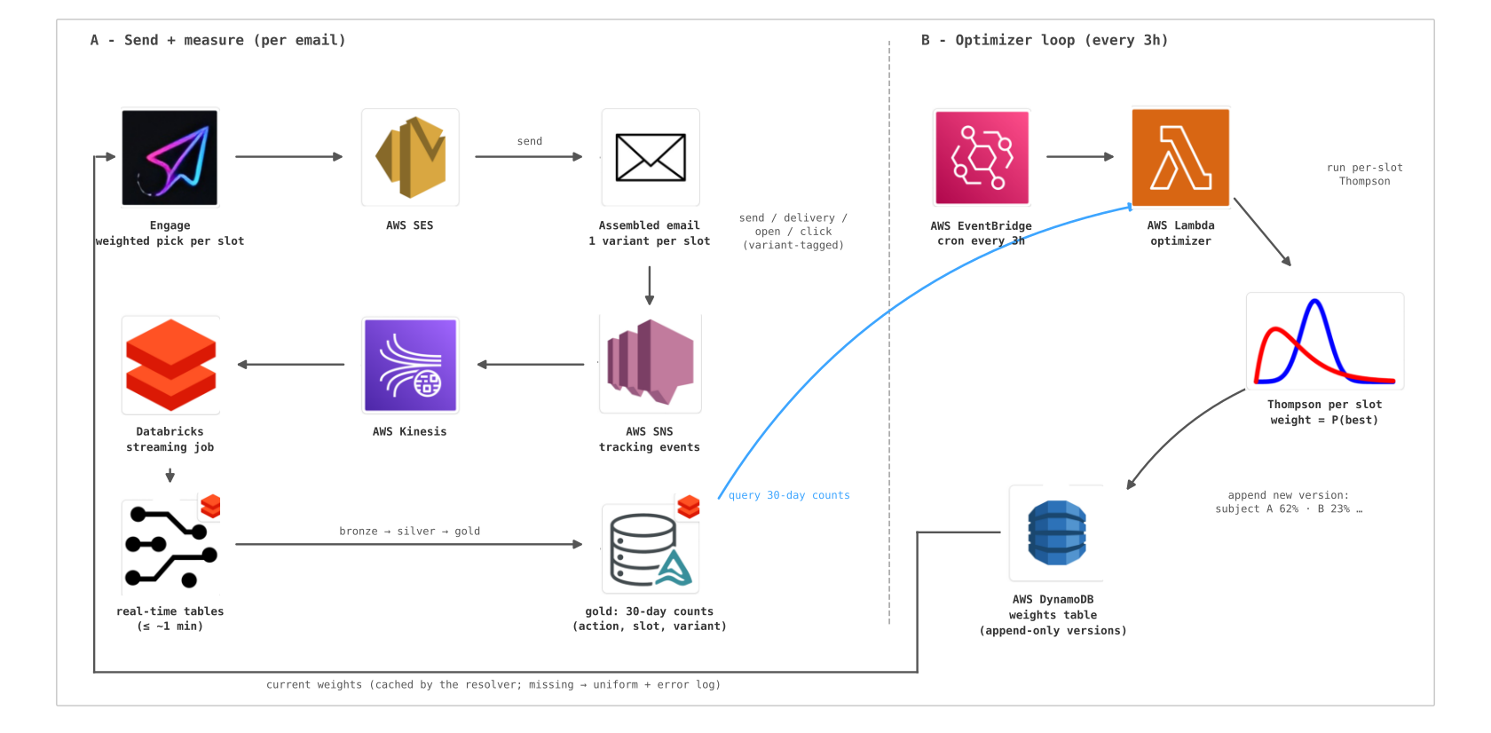
Reading those weights back is deliberately unbreakable - fail open: at send time the executor picks a variant through a cached resolver, and if the weights are missing or the read fails, it falls back to a uniform pick with an error log. The optimization layer can degrade a send to uniform (where every test starts anyway), but it can never block one.
Three things about the loop itself are worth calling out:
- It enumerates variants from the action, not from the data. This one is subtle and important: a variant that has received zero sends produces zero analytics rows - it's invisible in the performance data. If the loop derived the variant universe from the counts, a starved variant could never recover: no sends → no rows → no weight → no sends. The action payload is the source of truth for what exists; the counts are left-joined onto it, zeros and all.
- It is stateless. The loop never reads the previous weights - it recomputes the entire distribution from the accumulated counts every run. The previous weights are implicit in the data anyway (they shaped which variants accumulated sends). Stateless recomputation means no drift accumulation, no corrupted-state recovery procedures, and trivially reproducible runs.
- It ships with a kill-switch. A single flag runs the loop in compute-only mode: it logs the distribution it would write, without writing - so any algorithm change can prove itself against live production data before it owns a single send.
What We Have So Far
At this point the machine is assembled: templates with slots, per-slot variant pools, a weights table seeded uniform and owned by the loop, a fail-open resolver in the send path, a real-time measurement pipeline, and a scheduled, stateless feedback loop.
All that's missing is the algorithm that decides the numbers - and "turn counts into percentages" turns out to be a genuinely interesting design problem: the textbook answer is unstable in a subtle way, the stable answer ignores confidence, and the reward each slot should optimize is not the obvious one. That's Part 2. See you there.