
In Part 1, we built the machine: email templates with slots, per-slot variant pools, an append-only weights table, and a feedback loop that recomputes the allocation every few hours. This part is about the question at the center of it: how should that loop turn counts into percentages?
It sounds like a solved textbook problem - multi-armed bandits have canonical answers, and I covered the classic setup in the Multi-Armed Bandits post. But the textbook rarely mentions what happens when the allocation is a published product number, the reward arrives hours late, and two variants can be genuinely equivalent. So this is a field guide: the strategies that fit this problem, the math behind each, where they shine, and where they quietly break.
The Job Description
Every few hours, for every slot of every dynamic action, the optimizer receives each variant's 30-day counts - sent, opened, clicked - and must output one thing: a percentage allocation summing to 100. Judged against the realities of this system, a good rule has to:
- Converge: a genuinely better variant should end up with most of the volume.
- Stay stable under noise: the weights are stored, charted, and read by humans - a noise-level change in the counts should produce a noise-level change in the allocation.
- Calibrate exploitation to evidence: a 60/40 observed split backed by 200,000 sends deserves a harder bet than the same split backed by 2,000.
- Live with delayed, batched rewards: clicks trickle in for hours after a send, so there is no per-decision feedback - only a batch recompute over accumulated counts.
- Minimize knobs: every hand-tuned constant is a number someone must justify, revisit, and eventually get wrong.
No single rule gets all five for free. Let's hold the two serious candidates against the list.
Strategy 1: Probability Matching (Thompson Sampling)
The Bayesian answer. Give each variant a Beta posterior over its reward rate, built directly from its counts,
$$\theta_i \sim \text{Beta}(1 + \text{successes}_i,\ 1 + \text{failures}_i)$$
then allocate to each variant its probability of being the best: draw from all posteriors simultaneously (100,000 times) and count the share of draws in which each variant's rate comes out on top.
def allocate(slot):                       # one slot = one independent bandit
    if not passes_cold_start(slot):      # more on these gates below
        return uniform(slot.variants)
    a, b = posterior_params(slot)        # Beta(1 + successes, 1 + failures)
    draws = rng.beta(a, b, size=(100_000, len(slot.variants)))  # fixed seed
    p_best = share_of_draws_where_each_variant_wins(draws)
    return p_best * 100                  # weights sum to 100 per slot
Strengths. Exploitation is calibrated by confidence, and no knob does the calibrating. A clear winner's P(best) marches to ~100% exactly as fast as the evidence sharpens; statistically tied variants split near-uniformly; an under-sampled variant keeps winning some draws (its posterior is wide, so it sometimes samples high), which is exploration falling out of the math for free. And with a fixed random seed, the allocation is a pure function of the counts: same data in, same weights out.
Weakness - and it's a big one. Near a tie, P(best) thrashes. For two variants, the posterior probability that variant 1 beats variant 2 is approximately
$$P(\theta_1 > \theta_2 \mid \text{data}) \approx \Phi(z), \quad z = \frac{\hat{p}_1 - \hat{p}_2}{SE}$$
and when the true rates are equal, $z$ is a random walk hovering around zero, moving by noise-level amounts as counts accumulate. $\Phi$ maps those wanderings across most of the (0,1) interval: a $z$ drifting between $-0.8$ and $+0.8$ - pure noise - swings P(best) between 21% and 79%. More data does not fix this: the numerator and the standard error shrink together, so $z$ is scale-free; in the limit, for an exact tie, P(best) evaluated on fresh data is approximately uniformly distributed between 0 and 1. (It isn't Monte Carlo noise, either - at 100,000 draws the simulation error is a fraction of a percentage point. The jitter is in the data.) Here's the behavior on synthetic data - two variants with the same true click rate:
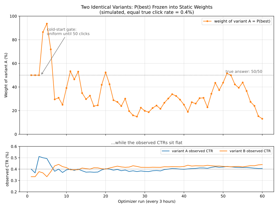
Whether this weakness matters depends on where the number goes. Near a tie it costs almost nothing in reward - if two variants perform the same, any split between them earns the same (hold that thought; it becomes the central insight of Part 3). But as a published number - stored, charted, and read daily by the campaign's owner - an allocation that says 80/20 today and 25/75 tomorrow over flat CTRs looks broken even when it isn't, and every metric computed downstream of the weights inherits the same instability.
Strategy 2: Proportional Allocation
The engineering answer. Score each variant by its posterior mean rate and allocate proportionally to a power of the score:
$$w_i \propto \max(\text{score}_i, 0)^{S}$$
The exponent $S$ dials the aggressiveness: $S = 0$ is uniform, $S = 1$ is plain proportional (a variant twice as good gets twice the weight), and $S \to \infty$ approaches winner-take-all. $S$ has to be hand-picked; a production-tuned value lands around $S = 6$.
Strengths. It is a smooth, deterministic function of the counts: a noise-level change in the data moves the allocation by a noise-level amount, by construction. Tied variants sit near uniform stably - the rule reports the tie instead of manufacturing a different winner every recompute. As a publishable number, it is perfectly behaved.
Weaknesses. $S$ is a magic constant - it encodes the entire exploration/exploitation trade-off by hand, and there is no principled way to choose it. Worse, the rule is blind to evidence volume: a 60/40 split in observed rates produces the same allocation whether it is backed by two thousand sends or two hundred thousand. Confidence - the very thing the Bayesian machinery exists to quantify - never enters the formula.
The two strategies side by side, run over the same simulated data - one variant with a genuine 20% relative edge - make the difference concrete:
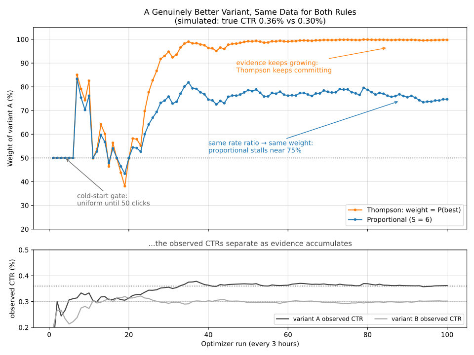
Both rules wobble while clicks are sparse - no allocation rule can outrun its data. The difference is what they do once the evidence firms up: Thompson keeps converting certainty into allocation - past 90%, past 95%, toward 100% - while proportional parks at whatever constant the observed ratio maps to (here ~75%) and stays there forever, shipping a quarter of the volume to a variant it has long known is worse. And whether that constant is 55% or 75% was decided by $S$, not by the data.
The Classics, and Why They Don't Fit
For completeness, the two standard bandit policies from the textbooks. ε-greedy (exploit the current leader; explore uniformly at random with probability ε) pays a permanent exploration tax on known losers and introduces yet another hand-tuned knob. UCB (deterministically pick the arm with the highest upper confidence bound) is built for choosing one arm per decision - it doesn't naturally produce a percentage split at all. The shape of this system - batch recompute, published static weights, delayed rewards - rules both out before their finer points even come up.
What Runs in Production: Thompson, Under Conditions
Probability matching wins the comparison - its confidence calibration is the property the whole feature exists for - but only under conditions that neutralize the instability:
- Cold-start gates. A slot stays at uniform weights until every variant has 500 sends - and, for click-based rewards, until the slot has accumulated 50 total clicks. The second gate matters more than it looks: confidence tracks clicks, not sends, and a slot can clear thousands of sends while carrying single-digit clicks, where every rate is noise.
- An accumulating window. Counts aggregate over a 30-day moving window, so between two runs three hours apart the data barely changes - and a deterministic function of slowly-changing counts changes slowly.
- A fixed random seed. Zero run-to-run Monte Carlo jitter; a weight change always means the data changed.
- A dense reward per slot - the next section, and the biggest single lever.
One honest caveat survives all of it: for truly equivalent variants, P(best) still drifts - just on the timescale of the 30-day window instead of every run. No allocation rule can settle a question the data can't answer. Recognizing that a permanently split P(best) means "this test is done, the variants are equivalent" takes a different statistic entirely - that's Part 3.
Choosing the Reward: Judge Each Slot on the Stage It Controls
What should "success" mean in those Beta posteriors? The natural answer - clicks, for every slot - is subtly wrong, and the reason is a funnel:
$$\underbrace{\frac{\text{clicks}}{\text{sends}}}_{\text{delivered CTR}} = \underbrace{\frac{\text{opens}}{\text{sends}}}_{\text{OR}} \times \underbrace{\frac{\text{clicks}}{\text{opens}}}_{\text{CTOR}}$$
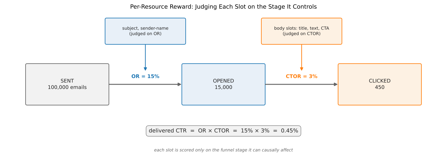
A subject line and a sender name do their entire job before the email is opened - their only causal path to a click runs through the open. The body slots (title, text, CTA) only exist after the open - they cannot cause one. So each slot is scored on the stage it causally controls:
| Slot | Reward | Posterior |
|---|---|---|
| subject, sender-name | Open Rate (OR) | $\text{Beta}(1 + \text{opened},\ 1 + \text{sent} - \text{opened})$ |
| body slots (title, text, CTA, ...) | Click-to-Open Rate (CTOR) | $\text{Beta}(1 + \text{clicked},\ 1 + \text{opened} - \text{clicked})$ |
Two independent arguments converge on this design:
- Signal density. Opens are roughly 50× more plentiful than clicks. A subject line scored on opens builds a sharp posterior in a fraction of the time it would need on clicks - the difference between a test that concludes in days and one that concludes next quarter.
- Confound removal. A body variant scored on plain CTR inherits the open rate of whatever subject it happened to be paired with. Since the body can't cause an open, that inherited variance is pure confound - a great CTA could lose its test for co-occurring with a weak subject line. CTOR conditions on the open and strips the confound out. Symmetrically, a subject scored on clicks could be punished for the sins of weak bodies downstream.
And since delivered CTR is exactly the product OR × CTOR, independently maximizing each factor maximizes the product: pick the best-opening subject and sender, pick the best-converting body, and the combination is the best delivered CTR the pools can produce. As a bonus, this makes Part 1's independence assumption tighter: slots optimized within separate funnel stages have less room to interact than slots all competing over the same end metric.
The Price of Caution: Penalty Terms and Guardrails
The objective of the whole system is blunt: maximize opens and clicks - the funnel rates each slot controls. Two well-intentioned additions tried to make the optimizer more careful than that, and both turned out to charge more than they returned.
The unsubscribe penalty. The obvious refinement is a cost-aware reward:
$$\text{score} = \text{click rate} - \lambda \cdot \text{unsub rate}, \quad \lambda = 5$$
(read: "one unsubscribe costs as much as five clicks gained"). The problem is that unsubscribes are rare - far rarer than clicks. Early in a test, with unsub counts of zero-to-a-handful per variant, the penalty is noise riding on almost no events, jittering the scores - and therefore the weights - for no informational gain. And by the time a campaign matures, every variant's unsub estimate has settled toward the same value, so the term shifts all scores by roughly the same constant and never flips a ranking. Noise early, a no-op late: the term came out. The reward stays exactly opens and clicks; unsubscribes are monitored outside the reward, where alerting belongs.
The guardrails. Floors and ceilings - "no variant below 1%, none above 95%" - existed for a defensible reason: keep some data flowing on every variant, so a wrongly-crowned early winner can still be dethroned by evidence. But look at where the bill lands: on the true winners, forever. With the floor in place, a slot's decided winner can never grow past ~95%. That reads like a modest 5% tax - until you remember there are five slots, each paying it independently. The share of emails assembled entirely from winners is
$$0.95^5 \approx 77\%$$
so nearly a quarter of all sends carry at least one component the data has already condemned - not during the learning phase, but permanently, on every converged test. And the insurance being bought with that volume was largely imaginary: replaying the allocator over real accumulated counts showed the floor pinning ~51% of losing variants above their true probability of being best - which, for a converged test, is very often ~0%.
So: no floor, no ceiling. A clear winner takes 100% of its slot; a clear loser goes to exactly 0%. The residual risk is real and worth writing down: a variant at 0% receives no traffic, so if the true ranking later reverses - seasonality, audience drift - the system cannot notice. That trade was made consciously: efficient by default, with the risk documented next to the constants.
Estimating the Lift - Without Overpromising
The last piece lives on the reading side, and it answers the user's real question: "what is this test buying me?" The product's headline number is the estimated CTR lift of the best combination (the top variant of each slot) over the default combination (the first-programmed variant of each slot - the email you'd have sent with no test at all). Under the same per-slot independence the optimizer assumes, per-slot gains multiply:
$$\text{lift} = \prod_{\text{slots}} \frac{\text{rate}_{\text{best}}}{\text{rate}_{\text{default}}} - 1$$
Multiplication is what makes this number exciting - five slots each just 5% better compound into a +28% combination - and also what makes it dangerous: any per-slot overestimate compounds just as eagerly.
And naive per-slot estimates overestimate wildly. A variant with 3 clicks on 100 sends has a raw rate of 3%; if the action's base CTR is 0.5%, that slot alone contributes "+500% lift" off what is essentially a coin-flip streak - and the argmax selects for exactly these flukes (the winner's curse: pick the max of noisy estimates and you'll usually pick the luckiest, not the best). Ship that raw number and the user watches a "+3,000% lift" melt into +12% over the following weeks. The test didn't get worse - the number was never real - but that's not how it feels, and it's the dashboard's credibility that pays.
The counter is empirical-Bayes shrinkage. Each variant's displayed rate is pulled toward the action's overall CTR $p_0$, with a prior worth $\kappa = 20$ clicks:
$$\tilde{p} = \frac{\text{clicks} + \kappa}{\text{sends} + \kappa / p_0}$$
A variant with no data reads exactly $p_0$ (zero lift). A variant with 3 clicks moves the needle a little. A variant with 300 clicks is barely shrunk at all - the data overwhelms the prior. The damping is continuous in the click volume, which beats a minimum-sample cutoff: there's no cliff where the number suddenly appears fully-formed and still noisy. And crucially, "best" is selected by the shrunk rate too, so a lucky low-click variant can't win a slot by chance.
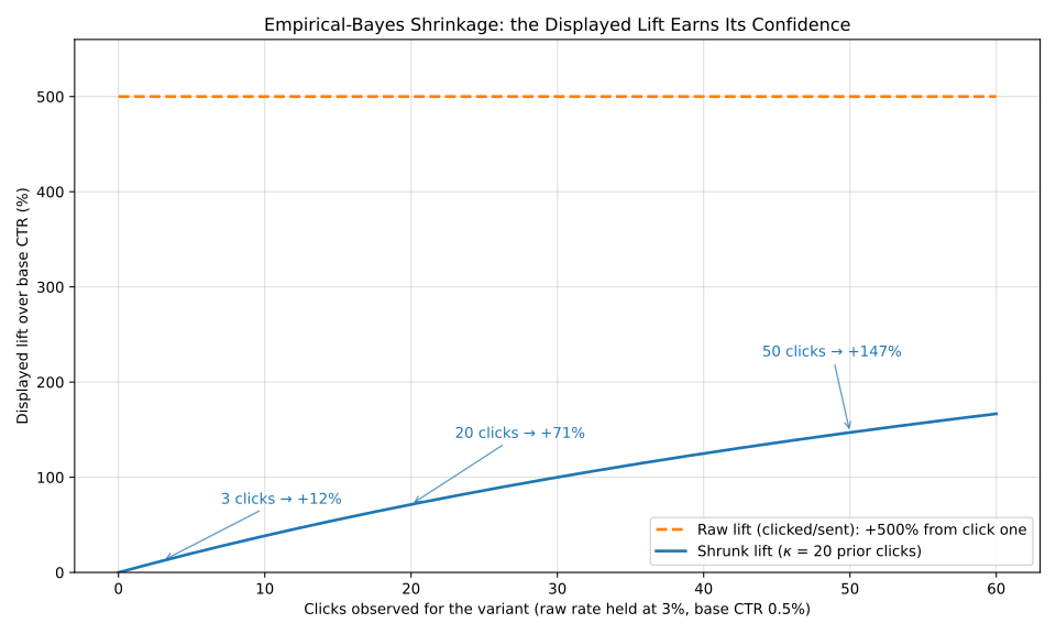
The displayed lift therefore under-promises early and converges to the truth as clicks accumulate - the right direction to be wrong in. A number that only ever grows into its promise builds trust; one that shrinks from it spends trust the product never gets back.
The Takeaways
- Calibration beats knobs. Probability matching under cold-start gates needs zero tuning to bet exactly as hard as the evidence supports; a sharpness exponent encodes the same trade-off as a number someone has to guess.
- Reward each decision on the stage it causally controls. The OR × CTOR decomposition buys more convergence speed than any tuning ever could.
- Insurance has a price - measure it. The floor's exploration benefit was mostly imaginary; its cost was real volume on condemned variants.
- Shrink anything you display. Raw ratios plus argmax equals winner's curse on a dashboard.
The allocator, then, is settled: probability matching, per-slot rewards, cold-start gates, no guardrails. But allocation only answers "where should the next send go?" Users ask a different question: "is my test done - can I ship the winner?" It turns out "done" needs its own statistic - expected regret - and that's Part 3. See you there.